Ncampbellmth212s09's Blog

Block 6

Hello and welcome to this the sixth and final block! Before we ship out for each, our own summer extravanganza’s there is one thing we need to discuss: Laplace Tansforms. This is a method created by a man named Pierre-Simon Laplace, to solve linear differential equations involving higher order derivatives. He realized that by transforming differential equations into algebraic equations, still with a degree of difficulty, it was possible to rearrange the algebraic expression and find a unique solution.

For this block we use Laplace transforms to discuss the general solutions of differential equations. In each case we will plot solution curves for a variety of parameters and given initial conditions. We are to discuss 2 examples of each of the following cases: First-Order, Second-Order and Linear Systems.

First-Order Equations

#1 p. 466

$\frac {dy}{dx} -y=e^{3t}, y(0)=2$

In order to plot the solution curve, I need to solve for a simple function of $y(t)$ . First I will take the Laplace Transform of both sides:

$\mathscr {L}[\frac {dy}{dx} - y]=\mathscr {L}[e^{3t}]$

Referencing our text, you can find derivations that simplify the left side of the equation, so it becomes:

$(s-1)Y(s)-2=\mathscr {L}[3^{3t}]$

As you can see I didn’t yet do anything to the right side. This much more complicated simplification is left to MATLAB’s built in function for solving a Laplace Transform $\mathscr {L}[x(t)]$ for a function $x(t)$ . The code for this is as follows:

>> laplace(exp(3*t),t,s)

ans =1/(s – 3)

This leaves us with:

$(s-1)Y(s)-2=\frac {1}{(s-3)}$

Solving for Y(s):

$Y(s)=\frac {2}{(s-1)} + \frac {1}{(s-1)(s-3)}$

We’re not done yet, remember we need to find $Y(t)$ not just $Y(s)$ . So to convert this equation into the time(t) domain I will use MATLAB’s built in inverse Laplace Transform function:

>> syms s t

>> ilaplace(2/(s-1)+1/((s-1)*(s-3)),s,t)

ans =exp(3*t)/2 + (3*exp(t))/2

That is…

$Y(t)=\frac {e^{3t}}{2} +\frac {3e^{t}}{2}$

There are a number of ways to plot equations in MATLAB. Gary showed my partner Paul and I the following method:

>> f=@(t) exp(3*t)/2 + (3*exp(t))/2

f = @(t)exp(3*t)/2+(3*exp(t))/2

>> fplot(f,[-1,1])

This produces the following plot:

6-1

#2 p. 466

$\frac {dy}{dt} +y=3cos(t), y(0)=-1$

$\mathscr {L}[\frac {dy}{dt}] +\mathscr {L}[y(t)]=\mathscr {L}[3cos(t)]$

You may notice the left side of the equation is very similar to the first example and can be transformed in the same manner. For the right side I will use MATLAB:

>> syms s t; laplace(3*sin(t),t,s)

ans = 3/(s^2 + 1)

Yielding:

$(s+1)Y(s)+1=\frac {3s}{(s^2+1)}$

Solving for $Y(s)$ :

$Y(s)=\frac{3s}{(s+1)(s^2+1)} -\frac {1}{(s+1)}$

Taking the inverse Laplce Transform using MATLAB:

>> syms s t; ilaplace(-1/(s+1)+3/((s+1)*(s^2+1)),s,t)

ans =1/(2*exp(t)) – (3*cos(t))/2 + (3*sin(t))/2

Leaving me with the equation with respect to time(t):

$Y(t)=\frac {3cos(t)}{2} -\frac {5}{2e^t} +\frac {3sin(t)}{2}$

Using the same “fplot” method as before I plotted this solution:

>> f=@(t)1/(2*exp(t)) – (3*cos(t))/2 + (3*sin(t))/2

f = @(t)1/(2*exp(t))-(3*cos(t))/2+(3*sin(t))/2

>> fplot(f,[-2,2])

6-2

The behavior of this graph isn’t as straitforward as the first example that just rose exponetially. So to get a better idea I’ll plot this again changing only the size of the window:

>> fplot(f,[-2,20])

6-2b

This is more clear that the solution falls into a regular cycle after the origin. This wave is due to the trigonometric functions implanted in the equations.

Second-Order Equations

#7 p. 466

$\frac {d^2y}{dt^2} +\frac {dy}{dt} -12y=0, y(0)=4, y'(0)=-1$

$\mathscr {L}[\frac {d^2y}{dt^2}] +\mathscr {L}[\frac {dy}{dt}] -12\mathscr {L}[y(t)]=\mathscr {L}[0]$

First simplifying to:

$\mathscr {L}[\frac {d^2y}{dt^2}] =s^2Y(s)-y(0)s+y'(0)$

Then to:

$s^2Y(s)-4s+1+sY(s)-4-12Y(s)=0$

Solving for Y(s):

$Y(s)=\frac {4s+3}{s^2+s-12}$

Taking the inverse Transform in MATLAB:

>> syms s t; ilaplace((4*s+3)/(s^2+s-12),s,t)

ans = (15*exp(3*t))/7 + 13/(7*exp(4*t))>> syms s t; ilaplace((4*s+3)/(s^2+s-12),s,t)

That is…

$Y(t)=\frac {12e^{3t}}{7} +\frac {13}{7e^{4t}}$

Plotting with the follwoing code yields the curve to this solution:

>> f=@(t)((15*exp(3*t))/7)+(13/(7*exp(4*t)))

f = @(t)((15*exp(3*t))/7)+(13/(7*exp(4*t)))

>> fplot(f,[-2,2])

6-3

Once again I’ll expand the window to get a better look:

6-3b

The solution equation contains two fractions, one with en exponetial function in the numerator and the other with one in the denominator. This accounts for the above graphical behavior, exponetial decrease leading to the origin then exponetial growth leaving it.

#11 p. 466

$\frac {d^2y}{dt^2} -8\frac {dy}{dt} +15y=6te^{4t}, y(0)=5, y'(0)=4$

$\mathscr {L}[\frac {d^2y}{dt^2}] -8\mathscr {L}[\frac {dy}{dt}] +15\mathscr {L}[Y(t)] =\mathscr {L}[6te^{4t}]$

Simplifying the left side as I had in the previous example and the left side using the following MATLAB code, I came up with the next equation:

>> syms s t;laplace(6*t*exp(4*t),t,s)

ans =6/(s – 4)^2

$s^2Y(s)-5s-4-8sY(s)+40+15Y(s)=\frac {6}{(s-4)^2}$

Solving for Y(s):

$Y(s)=\frac {6}{(s-4)^2(s^2-8s+15)} +\frac {5s}{s^2-8s+15} -\frac {36}{s^2-8s+15}$

Taking the Inverse Transform in MATLAB:

>> syms s t;ilaplace((6/((s-4)^2*(s^2-8*s+15))+(5*s)/(s^2-8*s+15)-36/(s^2-8*s+15)),s,t)

ans =(15*exp(3*t))/2 – (5*exp(5*t))/2 – 6*t*exp(4*t)

That is..

$Y(t)=\frac {15e^{3t}}{2} -\frac {5e^{5t}}{2} -6te^{4t}$

Plotting:

>> f=@(t)(15*exp(3*t))/2 – (5*exp(5*t))/2 – 6*t*exp(4*t)

f = @(t)(15*exp(3*t))/2-(5*exp(5*t))/2-6*t*exp(4*t)

>> fplot(f,[-2,2])

6-4

Linear Systems

#2 p. 470

$\frac {dx}{dt} +y=3e^{2t}; \frac {dy}{dt} +x=0$

$\mathscr {L}[\frac {dx}{dt}] +\mathscr {L}[Y(t)] =\mathscr {L}[3e^{2t}]$ and $\mathscr {L}[\frac {dy}{dt}] +\mathscr {L}[X(t)] =\mathscr {L}[0]$

Simplifying the first equations I get:

$Y(s)=\frac {3}{s-2} +2-sX(s)$

Then the second:

$X(s)=-sY(s)$

Solving the first equation for Y(s) using the definition of X(s) from the second equation and similarily X(s) using the definition of Y(s), I get the following two equations:

$Y(s)=\frac {3}{(s-2)(1-s^2)} +\frac {2}{1-s^2}$

$X(s)=\frac {-3s}{(s-2)(1-s^2)} -\frac {2s}{1-s^2}$

Taking the inverse transformof each in MATLAB:

>> syms s t;ilaplace((-3*s)/((s-2)*(1-s^2))-(2*s)/(1-s^2),s,t)

ans =1/(2*exp(t)) + 2*exp(2*t) – exp(t)/2

and…

>> ilaplace(3/((s-2)*(1-s^2))+2/(1-s^2),s,t)

ans =1/(2*exp(t)) – exp(2*t) + exp(t)/2

$Y(t)=\frac{1}{2e^t} -e^{2t}+\frac{e^t}{2}$

$X(t)=\frac{1}{2e^t} +2e^{2t}+\frac{e^t}{2}$

Plotting both equations:

6-5

The bottom line ( $Y(t)$ ) is decreasing at a slower rate then the top line( $X(t)$ ). The difference is increasing verses decreasing comes from the fact that in one equation $e^{2t}$ is positive and the other is negative. Also this term in the $X(t)$ equation is doubled compared to the $Y(t)$ equation, hence the difference in rates of change.

#5 p. 470

$latex \frac {dx}{dt} -5x +2y=3e^{4t}; \frac {dy}{dt} -4x+y=0$

$\mathscr {L}[\frac {dx}{dt}] -5\mathscr {L}[X(t)] +2\mathscr {L}[Y(t)] =\mathscr {L}[3e^{4t}]$

$\mathscr {L}[\frac {dy}{dt}] -4\mathscr {L}[X(t)] +\mathscr {L}[Y(t)] =\mathscr {L}[0]$

Simplifying and solving both equations simultaneously I got the following two equations in the s domain:

$X(s)=\frac {3(s+1)}{(s-4)(s-3)(s-1)} +\frac {3(s+1)}{(s-3)(s-1)}$

$Y(s)=\frac {12}{(s-4)(s-3)(s-1)} +\frac{12}{(s-3)(s-1)}$

Using MATLAB once again to take the inverse Laplace Transform, I got the following equtions in the time domain:

>> ilaplace((3*(s+1))/((s-4)*(s-3)*(s-1))+(3*(s+1))/((s-3)*(s-1)),s,t)

ans =5*exp(4*t) – 2*exp(t)

>> ilaplace(12/((s-4)*(s-3)*(s-1))+12/((s-3)*(s-1)),s,t)

ans =4*exp(4*t) – 4*exp(t)

latex X(t)=5e^{4t}-2e^t$

$Y(t)=4e^{4t}-4e^t$

Plotting:

6-6

The equations differ only slightly so this plot makes sense to me as the curves follow suit.

Well thats it I’m finished. Another semester done in the pursuit of success. I hope you enjoyed this as well as any of my other posts you may have checked out. For all the people stressin, remember: life isn’t a fact but more an opinion, so make sure you make your own. Also I’d like to give special thanks to a great man Gary Davis, if it wasn’t for him I wouldn’t have been able to return to my home in the green mountain state on the eighteenth instead hangin around for another final…so thanks Gary its been great- Take it easy…

Block 5

Systems of Linear Differential Equations. This statement is the topic of this the fith block of my MTH 212 career. To the untrained eye this phrase may seem to bare a horribly complex topic. Yet with the knowledge I have accumulated hence forth in my mathematical experience as an engineering student, the following concepts made perfect sense.

In the block I set out to analyze the behavior of a system of two linear differential equations. This pair of equations are in the forms:

$\frac {dx}{dt}=ax+by$

$\frac {dy}{dt}=cx+dy$

The first is the equation for the change in x, in terms of x and y, with repsect to a changing time(t). The second is similarly the equation for the change in y, in terms of x and y, with respect to a changing time(t). The symbols a, b, c and d represent values that in some situations can as well vary with time; but for our purposes in Block 5, we will keep them as constants. Our first objective is to analyze the linear function $T[(x,y)]=(x+y,x)$ , by plotting in two dimensions, as a vector field. This linear function can be broken up into the pair of differential equations like above:

$\frac {dx}{dt}=x+y$

$\frac {dy}{dt}=x$

Using the meshgrid function in MATLAB, I was easily able to make a two dimensional representation of this system. The code is as follows:

>> [x,y]=meshgrid(-1:1/10:1,-1:1/10:1);
>> u=x+y;
>> v=x;
>> quiver(x,y,u,v,1)

This yields the vector field shown here:

Each arrow represents the behavior of the linear function at that point. Remembering lower levels of my mathematical career, these vectors are line rays and theoretically continue on forever. But for the sake of analysis when plotting a vector field, it would become much to hectic to understand if each ray was drawn out. It is difficult to see many of the vector arrows in the section that runs from the upper left to bottom right of the grid. You can see on the plot all the arrows seem to diverge from this center area. To further understand the nature of the function we are to find the invariant lines for this system. An invariant line is one that does not vary in its path, that meaning it is constant making it linear. It seems to pass through to origin(0,0) so I was able to use the following precedure to solve for any invarient lines:

Knowing the relationship $T[(x,y)]= \lambda (x,y)$ , I begin by solving for the Eigen Values( $\lambda$ ). This relationship says that any vector of the line for which I’m solving is only different by the multiple $\lambda$ .

$(1-\lambda )x+y=0$ -> $x=\lambda y$

$x-\lambda y=0$ -> $y=-(1-\lambda )x$

Using the values of x and y in each others equations yields:

$(\lambda^2 - \lambda -1)x=0$
$(\lambda^2 - \lambda -1)y=0$

Since x or y mustn’t be zero in order to have line properties, I can divide one or the other out to solve for $\lambda$

$(\lambda -2)(\lambda -1)-1=0$ -> $\lambda = \frac {1}{2} (1\pm \sqrt {5})$

Plugging this into either of the original equations poses:

$y=(-1+ \frac {1}{2} (1\pm \sqrt {5}))x$

Therefore yielding the equations for the two invariant lines:

$y1=(\frac {\sqrt {5}}{2} -.5)x$

$y2=(-\frac {\sqrt {5}}{2} -.5)x$

Now plotting these in MATLAB using the following code, creates the graph below:

>> [x,y]=meshgrid(-1:1/10:1,-1:1/10:1);
u=x+y;
v=x;
quiver(x,y,u,v,1)
hold on
x=-1.5:.01:1.5;
y=-(1-.5*(1+sqrt(5))).*x;
plot(x,y)
x1=-0.8:.01:.8;
y1=-(1-.5*(1-sqrt(5))).*x1;
plot(x1,y1)

As was expected, one line runs from the top left to the bottom right, and both lines pass through the origin. With the other line it is easy to see the individual vectors along and near the invariant line are parallel. As you move from one line to the other you can see the vectors begin to transition from the direction of the one to the other. That explanation might have been a little confusing, think of it like this: the invariant lines are walls, you walk along the wall until you run into the other wall then you must turn and follow that wall. These walls are the true behavior of the linear function. All other vectors are influenced by these behaviors proportional to their proximity to each line respectively.

Next we were to experiment with a two different random assortments of constant values in the linear function form:

$T[(x,y)]=(ax+by, cx+dy)$ using values $-5 \leq a,b,c,d \leq 5$

First I decided to plot linear function:

$T[(x,y)]=(4x+y,2x+3y)$

I speculate that the whiter space running almost vertical in the middle of the plot will be an invariant line. Solving for any invariant lines present just as before yields the following two equations:

$y1=-3x$

$y2=x$

Plotting these lines on the mesh grid just as before poses:

Once again there are two lines, one of which runs down the whiter area and the other going from the bottom left to the top right. Both of course passing through the origin. In this plot unlike the first I looked at, has all vectors moving away from the origin. Next I’ll try a different combination of constants.

$T[(x,y)]=(-2x-5y,3x-4y)$

5_2

This comes out as a vector field spiraling anti-clockwise into the origin. Because all vectors seem to part of this spiral, there are no areas for a non-varying to run through.

Next I will move onto the second part of Block 5. In this part I will look at the six different geometric solutions: Stable Spiral, Unstable Spiral, Saddle, Stable Node, Unstable Node and Center. I will still using the characteristic equations as before:

$\frac {dx}{dt}=ax+by$

$\frac {dy}{dt}=cx+dy$

for the linear function corresponding to the matrix $A=\left (\begin {array}{cc} a&b\\ c&d \end {array} \right)$

Stable Spiral:

An example of a stable spiral was seen in my last plot. These types of functions have no real roots, meaning no real invariant lines. When I say there are no “real” roots I don’t mean there aren’t any roots, they just include the use of complex numbers( $i^2=-1$ ). What makes this a Stable geometry is because the vectors spiral in towards origin. This difference between stable and unstable will be easier to understand as I go through all the conditions. This specific scenario occurs when $\beta^2 -4\lambda<0$ .

$M=\left (\begin {array}{cc} -3&-3\\ 1&-4 \end {array} \right)$

stable_spiral

Unstable Spiral:

Like the last spiral there are no real roots which make for no real invariant lines. Since this condition is Unstable, the vectors will all spiral out away from the origin. If you think about it, the origin is the only place of invariation of a spiral. So then the defining factor of stability seems to come from whether or not the system converges on such area of invariation. This specific condition occurs when $\beta^2 -4\lambda<0$ , $\lambda = ad-bc$ and $\beta =a+d$ .

$M=\left (\begin {array}{cc} 5&-4\\ 1&4 \end {array} \right)$

unstable_spiral

Saddle:

A “saddle” is a point a characteristic of a graphical solution when there is a point of relative maximum or minimum of the saddle point but not of the entire solution. The name comes from the behavior on a graph looking similar to a saddle used on a horse. This specific condition occurs when $\lambda >0$ and $\beta<0$ .

$M=\left (\begin {array}{cc} -3&1\\ 2&1 \end {array} \right)$

Solving for the invariant lines as before yields the equations:

$y1=(2+\sqrt {6} )x$

$y2=(2-\sqrt {6} )x$

Stable Node:

A stable node may at first seem like a stable spiral, but unlike the spiral there is one invariant line. This area is know as the equilibrium point and being a stable solution all vectors are oriented towards it.

This specific situation occurs when $\lambda >0$ and $\beta<0$ .

$M=\left (\begin {array}{cc} -3&1\\ -2&0 \end {array} \right)$

stable_node

Solving for the invariant line I found:

$y=x$

Unstable Node:

Since this is Unstable the vector flow will be away from the equilibrium point. This specific situation occurs when $\lambda >0$ and $\beta>0$

$M=\left (\begin {array}{cc} 4&1\\ 3&2 \end {array} \right)$

Solving for the invariant lines I found:

$y1=-3x$

$y2=x$

Center:

This form is very similar to the spiral. There are no real invariant lines as all vectors are behaving in varying ways. The major difference in this type of solution is that instead of being Stable or Unstable, the vectors seem to spiral, orbiting the origin. This specific situation occurs when $\lambda >0$ and $\beta=0$

$M=\left (\begin {array}{cc} 1&-2\\ 1&-1 \end {array} \right)$

center

To me this seems much more then the stable spiral, but hey that’s just me. Well that’s enough for this block. I hope you’ve enjoyed it. Until next time…take it easy.

Block 4

Block 3

Do you know this guy? You should. His name is Edward Lorenz and he’s the guy that created a simplified method of of modeling convection rolls that come about in equations describing atmospheric activity. Heck yeah he did. He published this paper Deterministic Nonperiodic Flow in the Journal of Atmospheric Sciences in 1963. This paper gave the basis for the eventual Chaos Theory. Whats the point of this history lesson? Well in order to model such physical and biological phenomena, you must use systems of differential equations. And these systems are the topic of the this the third block.

Lorenz’s method was made up of the following three equations:

$\frac{dx}{dt} = \sigma (y - x)$

$\frac{dy}{dt} = x (\rho - z) - y$

$\frac{dz}{dt} = xy - \beta z$

These three linked differential equations include the three parameters σ, ρ, and β are all positive. σ is called the Prandtl Number and β is known as the Rayleigh Number. Both of these postive paremters pertain to the physical properties of a fluid in motion. Most commonly they are set to σ = 10 and β = 8/3. Varying the values of ρ yield qualitativly differing solution curves for a specific system. Setting ρ = 28 you get what has come to be known as the lorenz attractor. This solution curve which looks similar to an opened zebra mussle, is said to be chaotic as all nearby points diverge almost exponentially rapid.

The objective of this the third block is to further our exploration of the Euler method of approximation by applying it to systems of differential equations. I will do this by comparing exact solutions to the Euler approximations. Specifically I will experiment with various paremters in both the Lorenz and Rössler Systems of differential equations.

The Euler Method M-file I had used for previous blocks is null and void to this block since we are now discussing systems verses just a single differential equation. The code for this new M-file is as follows:

% Euler’s method for a system of differential equations.

% The differential equations are dy/dt = f(t,y) where y is a vector of unknown functions.

function [ t, y ] = euler_system( f, t_range, y_initial, nstep )

% We set a range of time values, from t(1) to t(2).

t(1) = t_range(1);

% We define dt by dividing the time range into an equal number of specified steps.

dt = ( t_range(2) – t_range(1) ) / nstep;

% We set the initial value of the vector y at the beginning time t(1).

y(:,1) = y_initial;

% We use Euler’s method to update the value of y at new time steps.

% “feval” is used instead of “eval” because we are passing the name of f to the program.

for i = 1 : nstep
t(i+1) = t(i) + dt;
y(:,i+1) = y(:,i) + dt * feval ( f, t(i), y(:,i) );
end

% The following command plots the components of y as functions of t.

plot(t,y)

% We also want a 3D plot of the vector components as they vary with t.

plot3(y(1, : ),y(2, : ),y(3, : ))

Saving this as euler_system.m I could then use it to plot both 2D and 3D approximations. Next I needed to create another m-file as done before, to specify the argument for the euler_system.m file to approximate. First I analyzed the Lorenz equations making the following code:

function yprime = lorenz_system ( t, y )
yprime = [ 10.0* (y(2)-y(1)); y(1)*(28.0-y(3))-y(2);y(1)*y(2)-(8/3)*y(3) ];

The three bolded numbers are the values inputed for σ, ρ, and β respectively. To then produce the 2D and 3D plots I had to input the following code into the MATLAB command window. The range of t values is set from 0-20 and the needed number of steps is set to 1000.

>> y_init = [ rand(); rand(); rand() ];

>> [ t, y ] = euler_system ( ‘lorenz_system’, [ 0.0, 20.0 ], y_init, 1000 );

The code produces the following two graphs:

2D Euler:

block3a

3D Euler:

block3b

The first 2D plot is very chaotic, having no real pattern to its curves. The blue and green lines as are closly related in that they follow pretty much the same path at an approximately constant deviation. The red line on the other hand differs greatly in value and though at first might look symmetric after closer examination is fairly independant of its counterparts paths. The 3D plot exemplifies mathematical entropy. The two dual spiral created is in no aspect uniform. The values diverging exponetially create a spirally effect that shifts planes as closes inward. Notice each ring in the spiral are at different spacing, with no inclination towards convergence or divergence. Next I will see how an ode45 solution will compare.

First I created an M-file denoteing the variables σ, ρ, and β:

function xdot = g(t,x)

xdot = zeros(3,1);

sig = 10.0;

rho = 28.0;

bet = 8.0/3.0;

xdot(1) = sig*(x(2)-x(1));

xdot(2) = rho*x(1)-x(2)-x(1)*x(3);

xdot(3) = x(1)*x(2)-bet*x(3);

Next I created an M-file to run this prior g.m file in an ode45 function:

function lorenz_demo(time)

% Usage: lorenz_demo(time)

% time=end point of time interval

% This function integrates the lorenz attractor

% from t=0 to t=time

[t,x] = ode45(’g’,[0 time],[1;2;3]);

disp(’press any key to continue …’)

pause

plot3(x(:,1),x(:,2),x(:,3))

print -deps lorenz.eps

3D ode45:

block3c

Remembering that in these examples, ρ =28 meaning the solution was to be chaotic. Ode45 produces this very similar dual spiral solution as had Euler’s. There are many more rings in each spiral making it look more uniform but In reality it is just as chaotic. Having more lines at this scale just makes it nearly impossible to see specific portions of curves. The reason there are more values involved is that ode45 has a much larger time range then Eulers method uses. This makes for a more exact solution in most cases but because this solution is chaos, it merely just produces more values.

Using the same two methods of analysis, that is; the same codes, I’ll see how switching the ρ value effects the solution. Setting ρ = 8, I produced the follwowing plots:

Euler 2D:

lorenzeuler2d

Euler 3D:

lorenzeuler3d

ode45 3D:

lorenzode3d

In the 2D plot the red line has very similar behavior to that of the blue and green. All three lines rather quickly converge to a single dimension(only one varying value). In the 3D plots, this same convergence can be scene by the single relatively uniform spiral. The ode45 spiral this time has less rings and is more of a consistant inward spiral then the less accurate Euler apporximation. The Euler spiral pinches at the bottom, in proximity to the set initial value of the origin. Yet the portion of spiral away from this initial point is more arcing. I interpret this as an example of Euler’s Methods flaws. From this comparison I can see that decreasing the value of ρ allows for more order in approximating a solution.

Next I will move on to experimenting with a Rossler system of differential equations. The equations are as follow:

$\frac{dx}{dt}=-y-z$
$\frac{dy}{dt}=x+ay$
$\frac{dz}{dt}=b+z(x-c)$

These are all ordinary non-linear differential equations that define a chaotic system that varies over a time interval Δt. These equations are defined by the parameters a, b and c. Rössler studied the attractor created by these equations with the parmeters set to: a=0.2, b=0.2 and c=5.7. This Rössler Attractor is pictured below(image provided by wikipedia.org):

Most of the spiral is in the xy plane. This is because only two of the equations are influenced by values in the z-direction. Furthermore when z=0 the two equations become linear and the other is a constant. This allows for easy analysis in only the xy plane. I would have to assume aswell from my new knowledge of the first order nature of Eulers approximation that when z=0 a solution will be more easily and accurately estimated. Notice how in the xy-plane the spiral seems to be about an approximate center, but then all the portion extruded into the z-direction twists and defines a different point of reference. This change happens as the x and y values spiral in towards the origin(0,0), allowing the z variable to have more influence of the behavior. While obtaining the wonderful image from wikipedia I read that the values a=0.1, b=0.1 and c=14 are of the most common in use of the Rössler system. I will follow the same procedure as before with the lorenz equations. Using the same euler M-file, I then need only to redefine the equations and their respected parameters.

The new function M- file is:

function yprime = rossler_system ( t, y )
yprime = [-(y(2))-y(3);y(1)+(0.2*y(2));0.2+(y(3)*(y(1)-5.7))];

Once again I made the set parameter values bold to make is easier for you my reader to pick them out. In this first attempt I am using the same parameters Rössler used in his study. Inputing the following command into MATLAB will produce a 2D and 3D solution curve.

>>y_init=[ rand(); rand(); rand() ];
>>[ t, y ] = euler_system ( ‘rossler_system’, [-50.0, 50.0 ], y_init, 10000 );

Euler 2D:

ross2d1

Euler 3D:

ross3d

In the 2D plot, the green line seems to be slightly ahead of the blue line but their overall behavior is equivalent. The red line is similar in that it spikes when the largest ocsillations occur in the other lines. The overal behavior of either line is highly chaotic. The only pattern that could be put to it is a repeating progression of increasing amplitude which resets at differents values over seemingly un related intervals. The 3D plot is a Rössler Attractor like the previous image. Eulers method produces very few curves but the rebelous nature of the z-orbitals can still be viewed. I saw when analyzing the Lorenz Attractor, ode45 produce more curves with such levels of chaos. So my next step is to creat two new M-files. First to denote the equations and their parameters then to run that file in an ode45 function.

rossler.m:

function xdot = rossler(t,x)

xdot = zeros(3,1);

a = 0.2;

b = 0.2;

c = 5.7;

xdot(1) = -(x(2))-x(3);

xdot(2) = x(1)+a*x(2);

xdot(3) = b+x(3)*(x(1)-c);

ode45.m:

function rossler_demo(time)

[t,x] = ode45(’rossler’,[0 time],[1;2;3]);

disp(’press any key to continue …’)

pause

plot3(x(:,1),x(:,2),x(:,3))

print -deps rossler.eps

Then inputting the following command into MATLAB will produce the desired plot.

>>rossler_demo(200)

ross3d21

My assumption was correct. Ode45 produced created a greater number of approximations. Recalling that ode45 is a 4th order method of approximation compared to Euler’s which is a first order, this situation seems appropriate. Also the fact that ode45 is being solved over the time range 0-200 where as the euler is -50-50; makes for a created number of curves in its plot. Regardless both solutions seem t gravitate around the same two approximate areas. Finally I am going to test what will happen if I change all three parameters. I noticed most of the talked about sets of parameter values puts c equal to a much higher number then a and b. Since we already saw that a high ρ value in the lorenz equations yields greater chaos, I thought I’d try a c value in the same area as a and b. My partner Paul Hannah and I decided to just pick three completely arbitrary values that were all less then 1. The values and code are as follows:

a=0.7 b=0.11 c=0.54

rossler_systerm.m

function yprime = rossler_system ( t, y )
yprime = [-(y(2))-y(3);y(1)+(0.7*y(2));0.11+(y(3)*(y(1)-0.54))];

MATLAB Command:

>>y_init=[ rand(); rand(); rand() ];
>>[ t, y ] = euler_system ( ‘rossler_system’, [ 0.0, 10.0 ], y_init, 5000 );

Euler 2D:

rosslar2d

Euler 3D:

rossler

rossler.m:

function xdot = rossler(t,x)

xdot = zeros(3,1);

a = 0.7;

b = 0.11;

c = 0.54;

xdot(1) = -(x(2))-x(3);

xdot(2) = x(1)+a*x(2);

xdot(3) = b+x(3)*(x(1)-c);

ode45.m:

function rossler_demo(time)

[t,x] = ode45(’rossler’,[0 time],[1;2;3]);

disp(’press any key to continue …’)

pause

plot3(x(:,1),x(:,2),x(:,3))

print -deps rossler.eps

MATLAB Command:

>>rossler_demo(15)

rossler2

Looking at the 2D Euler approximation you can instantly see that there is very little if any structure in the lines. That fact plus the magnitude of lines involved in the ode45 solution lead me to believe that decreasing the c value does not necessarilly lead to greater order. Furthermore the Euler 3D plot seems to be almost linear on the bottom of the cornucopia shaped spiral. The ode45 plot seems to be more consistant in its spiralling. I believe this can be again attributed to the difference in the methods of approximation. Where the Euler aproximation seems linear in the spirally is due to it’s first order method of estimating solutions plus the fact that its occuring around z=0. As you can recall from earlier in this, my Block 3 blog, I discussed that when z=0, the equations become linear:

$\frac{dx}{dt} = -y$

$\frac{dy}{dt} = x + ay$

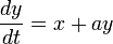
With the third being constant at b.

So with now three blocks completed, I look excitedly on to my future in this exploration of differential equations. Remembering of course, the information already obtained. This isn’t difficult though, as many of the main ideas continue to be examined in each of our blocks. Idea’s such as understanding types of approximation methods makes analysis an easier process. Well I hope you’ve enjoyed “Block 3” brought to you by Nick Campbell. An extra happy Patriots Day to everyone! Until next time, take it easy…

Block 2

Aloha! Here in this, my second block wordpress blog, My partner Paul Hannah and I are going to continue our analysis of numerical approximations for differential equations. Last block I got familiar with the Euler method of approximation. This technique is referred to as a first order method. This means its uses strait lines to make up an estimate of the solutions slope. In non graphical terms this means the error between the exact and approximate solution is merely a constant time the set step size. This error is represented by the statement:

|y_i-y(x_i)|≤Ch

Where C is a constant value depending on the function and specific interval and h is the step size, as explained in the text. Unfortunately things aren’t always constant which in turn cause Eulers method to be prone to errors. Knowing this, two mathmeticians Carl Runge and Wilhelkm Kutta set out to create a better way. What they came up with is known as the Runge-Kutta 4th Order Method. The fact that this was a 4th order approximation meant that instead of using a bunch of strait lines to make up a solutions curve, they used parabolas and quartics. This in turn makes for a much more accurate approximation:

|y_i-y(x_i ) |≤Mh^4

Where M is a constant value depending on the function and specific interval and h is the step size, as explained in the text.

To begin I used the same technique of creating m-files for the differential equation and Euler method. The Euler file was still on the computer I had been using so it was unnecessary to save a new version. To experiment with the new concept of implementing the Runge-Kutta method I began with a simple problem. MATLAB has a built in function called “ode 45” that is used like the Euler m-file. Though question 1 was not included in the assignment I chose to try it first since it was a simple equation.

Problem 1: pg 138: dy/dx=x^3

function yprime=problem1(x,y)

yprime=x^3

>> [x,y]=ode45(‘problem1’,[0,1],0)

>> plot(x,y)

problem1

Next I tried graphing this with plotting this with the Euler approximation. In order to do this you need to add “hold on” and “hold off” surrounding the plot commands. Also notice the ‘r:’ in the second plot command. This tells MATLAB to make that line red and dotted. This helps differentiate between the lines if they come out very close.

>> [x1,y1]=ode45(‘problem1’,[0,1],0);

>> euler3(‘problem1′,[0,1],0,50);

>> hold on

>> plot(x1,y1);

>> plot(x,y,’r:’);

>> hold off

problem1e

Its difficult to see but there is a slight difference between the two approximations. Since this was such a simple problem both methods pose a “good enough” solution.

MATLAB also has a built in function of solving first order differential equations that do have an exact solution. This is called “dsolve”. You can see that the answer produced is simply the indefinite integration of the equation with respect to x.

>> dsolve(‘Dy=x^3′,’x’)

ans = x^4/4 + C2

Problem 2:Pg. 138 dy/dx=(x^4)*y, y(1)=1

>> dsolve(‘Dy=x^4*y’,’x’)

ans = C4*exp(x^5/5)

Here dsolve differs from the explicit solution given in the book, this may elude to fact that there is not an exact solution.

The great man that he is, Eric Sykes devised the following code that plots the Euler method(red), ode45(blue) and explicit solution(green). Putting these all together will show which approximation method best suits the problem.

[x,y]= Euler1(’Example’,[1,2],1,.1);
[x2,y2]= ode45(’Example’,[1,2],1);
x3=1:.1:2;
y3= exp((x.^5-1)/5);
hold on
plot(x,y,’r’);
plot(x2,y2,’b’);
plot(x3,y3,’g’);
hold off

problem2-graph

The graph generated evinces quite clearly that the Euler is inferior to ode45. Up to x=1.6 (about), all three lines close. Yet as they continue Euler quickly strays off while ode45 stats relatively close. Also this is such a great example because you can see how the Euler approximation is much more linear as the ode45 is a smooth curve. Almost to smooth of a curve as the explicit solution looks linear up against it. This difference most likely come from the fact that ode45 uses parabolas and quartics which are even order equations and the explicit solution is an odd order equation.

Problem 3: Pg. 138: dy/dx=-y^2cos(x), y(0)=1

>> [x,y]=ode45(‘problem3’,[0,pi],1)

>> [x2,y2]=euler1(‘problem3′,[0,pi],1,.1)

>> hold on;
>> plot(x,y,’b’)
>> plot(x2,y2,’r’)
>> hold off

In the generated graph, Eulers method once again begins similar to the ode45 curve but quickly diverges.

>> dsolve(‘Dy=-(y^2)*cos(x)’,’x’)

ans =

-1/(C3 – sin(x))
0

Problem 6:Pg. 139: dy/dx=xy^2, y(0)=1

>> [x1,y1]=euler1(‘problem6’,[0,1],1,.1);
>> [x2,y2]=ode45(‘problem6′,[0,1],1);
>> hold on
>> plot(x1,y1,’r’);
>> plot(x2,y2);
>> hold off

problem6

>> dsolve(‘Dy=x*y^2′,’x’)

ans = -1/(x^2/2 + C3)

Problem 10:Pg. 139: dy/dx=x+y, y(0)=0

>> [x1,y1]=euler1(‘problem10’,[0,1],1,.1);
>> [x2,y2]=ode45(‘problem10′,[0,1],1);
>> hold on
>> plot(x1,y1,’r’);
>> plot(x2,y2);
>> hold off

problem-10-graph

>> dsolve(‘Dy=x+y’,’x’)

ans =

C3*exp(x) – x – 1

Problem 13:Pg. 139: dy/dx=(x^3)*y+(x^2)(y^2), y(-1)=1

>> [x1,y1]=euler1(‘problem13’,[0,1],1,.1);
>> [x2,y2]=ode45(‘problem13′,[0,1],1);
>> hold on
>> plot(x1,y1,’r’);
>> plot(x2,y2);
>> hold off

problem13-graph

Its interesting to see in this graphical approximation the two methods diverge as they had in the other examples but then converge and cross just after x=.9. This looks to be again the fault of the methods fundamental difference. Because the euler method is a first order approximation it cannot change direction as smoothly as the fourth order curve and thus intersects it.

>> dsolve(‘Dy=((x^3)*y)-((x^2)*(y^2))’,’x’)

ans = 1/(C9/exp(x^4/4) + int(x^2*exp(x^4)^(1/4), x)/exp(x^4/4))

Problem 16: Pg. 139: y*(((x^2)+(y^2)+1)^(1/2))+cos(x*y), y(0)=1

>> [x1,y1]=euler1(‘problem16’,[0,.01],1,.001);
>> [x2,y2]=ode45(‘problem16′,[0,.01],1);
>> hold on
>> plot(x1,y1,’r’);
>> plot(x2,y2);
>> hold off

problem16-graph

At first I got an obviously incorrect graph as the lines were horizontal and vertical. So I then changed the step value to .001 from .01 and x interval from [0,.1] to [0,.001] to generate the above graph. This still seemed perculiar so I entered the dsolve and found as follows:

>> dsolve(‘Dy=(y*(((x^2)+(y^2)+1)^(1/2)))+cos(x*y)’,’x’)
Warning: Explicit solution could not be found.
> In dsolve at 156

ans =

[ empty sym ]

This means there is no exact solution and is why a proper approximation wasn’t working out.

In the end I feel I have learned alot and really grown as an individual functioning in modern society. But it is in these times of revelation, I realize: how far I’ve come is really only measurable by how far I have yet to go and when the skies the limit-well, I’ve got alot more work to do. So I go now onto block three. I hope you enjoyed my Block 2 Blog, take it easy-Aloha.

First Block

Whats up party people. As engineers we usually need to visually interpret data in order to fully understand and believe in it. This is why I’m sure many of us weren’t to surprised upon discovering santa clause wasn’t real and is why in order to learn about differential equations we began with graphical analysis. The concept of a solution is slighty different in regard to differential equations. More commonly a solution is arriving at a single point or quantity. Differential equations pose solutions of much more information. This is why we need to analyze them graphically by plotting what is called a directional field using MATLAB. This will show overall trends of the equations solution. To further this understanding we will then use a technique of numerical approximation known as Eulers (pronounced “oilers”) Method. This generates a single trend line of the solution. When placed over the directional field this line should follow the general flow of the graph…hopefully.

I’ll begin with problem 18 from chapter two in “A Course in Ordinary Differential Equations”, our classes text. The following code was influenced by Gary Davis’s famous “first block details” blog.

Problem 18(p. 94): dy/dx=x+y

>> [X,Y]=meshgrid(-2:0.4:2,-2:0.4:2);

>> DY=X+Y;

>> DX=ones(size(DY));

>> DW=sqrt(DX.^2+DY.^2);

>> quiver(X,Y,DX./DW,DY./DW,0.5,’.’);

>> xlabel(‘x’);

>> ylabel(‘y’);

You can see where each value passes either of the x=0 axis or y=0 axis the field lines shift from negative slope to postive slope. I feel like this trend continues so I decided to expand the dimensions of the plot. You can see this change in the MATLAB code, first line after “meshgrid”.

>> [X,Y]=meshgrid(-5:0.25:3,-1:0.25:4);
>> DY=X+Y;
>> DX=ones(size(DY));
>> DW=sqrt(DX.^2+DY.^2);
>> quiver(X,Y,DX./DW,DY./DW,0.5,’.’);
>> xlabel(‘x’);
>> ylabel(‘y’)

derka

Here you can see how as you move away from zero, the field lines gradually move to a vertical position. Next we will use Eulers Method of numerical approximation. To do this we’ll set up an m-file in MATLAB which contains the code for Eulers Method. By doing this we’ll be able to just enter a reference to the m-file instead of having to type it each time it is used. The code for the m-file is as follows:

function [ x, y ] = euler ( f, x_range, y_initial, nstep )

dx = ( x_range(2) – x_range(1) ) / nstep;

x=zeros(nstep+1,1);

y=zeros(nstep+1,1);

for i = 1 : nstep
x(i+1) = x(i) + dx;
y(i+1) = y(i) + dx * feval ( f, x(i), y(i) );
end

plot(x,y)
xlabel(’x’)
ylabel(’y’)

After saving that we then made another smaller m-file to specify what equation was being used:

function yprime = example1(x,y)
yprime = x+y;

Now that you have these two m-files you implement them in the MATLAB command window by entering:

>> euler(’example1′,[0,6],1,60)

This tells the program to use Eulers method on problem 18(saved as ‘example 1’ ) with an x-range from zero to six, a y-intial of one and a step size of sixty. Below is the graphical result of this process. As you can see the line transistions to a vertical postition as is moves away from the origin.

eulerp1a

Next we’ll take this trendline and post it into the directional field. I feel that Emile Tayeh from section 1 portrayed it best on his first block post when he generated this graph:

combined

Notice how the line follows the trend of the field? The field lines run tangent to the numerical approximation. This makes sense as differentiating an equation yields the slope of that equations tangent line. Whether this is an accurate assumption or not it seems to me that this numerical line is the directional field’s integral. The MATLAB code to produce this representation is as follows.

>>[x,y]=euler(’example1′,[0,1],1,120)

>> [X,Y]=meshgrid(0:0.5:12,0:0.5:18);

>> DY=x+y;
>> DW=sqrt(DX.^2+DY.^2);
>> quiver(X,Y,DX./DW,DY./DW,0.5);
>> hold on
>> plot(x,y)

>> hold off
>> xlabel(’x’)
>> ylabel(’y’)

As you can see this is just combining the two code sequences we have already explored.

Now to ensure that we understand what we just did, Gary assigned another equation, . We will use the same techniques used in the previous example except now the equation is in terms of “t” instead of “x”. This change of variable for our present purposes is meaningless. Though this was a simple change you can view the error I intitially made when assigning axis labels. I entered “tlabel” where “xlabel” was needed. I was just worried about changing all the x’s to t’s, not realizing that such code was refering to the cartesian coordinate system where x is horizontal and y is vertical.

>> [T,Y]=meshgrid(-4:.5:4,-4:.5:4);
>> DY=(Y.^2+T);
>> DT=ones(size(DY));
>> DW=sqrt(DT.^2+DY.^2);
>> quiver(T,Y,DT./DW,DY./DW,0.5,’.’);
>> tlabel(‘t’);
??? Undefined function or method ‘tlabel’ for input arguments of type ‘char’.

>> xlabel(‘t’)

>> ylabel(‘y’)

This plot may seem slightly more random then the last so lets continue and apply the Euler Method of numerical approximation. In only modifying the variables and intervals of the previously used MATLAB code we get:

eulerp2a

As you may notice, the intervals presented in the last graph were much smaller then that of the directional field, this is to best view the trend of the solution. Keeping these smaller intervals, the trend line matches up beautifully with the directional plot. Look at the point (-1,-1). This is a perfect representation of the field line being tangent to the approximation.

eulerp2b1

In the end of it all I have learned some basics on the operation of MATLAB, how to plot differential equations and what Eulers Method is. Personally I don’t feel Eulers Method is affective at all. Most likely it may be myself missing an essential piece of information, but it seems like the trends created are almost to specific and are not the best representation of the entire field. The two problems I explored were very simple . I’m almost positive that presented with a more complex equation Eulers Method would be even less accurate. But hey I don’t mean to come off as unappreciative, from what I’ve heard he seemed like a good fellow. Anyway thats enough for now, take it easy.

Hello world!

Welcome to WordPress.com. This is your first post. Edit or delete it and start blogging!

Ncampbellmth212s09’s Blog

Block 6

First-Order Equations

Second-Order Equations

Linear Systems

Block 5

Block 4

Block 3

Block 2

First Block

Hello world!

Pages

Categories

Archives

Search

Blogroll

RSS Feeds

Meta